Refining posterior estimates with importance sampling

Theory

SBI estimates the posterior \(p(\theta|x) = {p(\theta)p(x|\theta)}/{p(x)}\) based on samples from the prior \(\theta\sim p(\theta)\) and the likelihood \(x\sim p(x|\theta)\). Sometimes, we can do both, sample and evaluate the prior and likelihood. In this case, we can combine the simulation-based estimate \(q(\theta|x)\) with likelihood-based importance sampling, and thereby generate an asymptotically exact estimate for \(p(\theta|x)\).

Importance weights

The main idea is to interpret \(q(\theta|x)\) as a proposal distribution and generate proposal samples \(\theta_i\sim q(\theta|x)\), and then augment each sample with an importance weight \(w_i = p(\theta_i|x) / q(\theta_i|x)\). The definition of the importance weights is motivated from Monte Carlo estimates for the random variable \(f(\theta)\),

\[ \mathbb{E}_{\theta\sim p(\theta|x)}\left[f(\theta)\right] =\int p(\theta|x) f(\theta)\,\text{d}\theta \approx \sum_{\theta_i\sim p(\theta_i|x)} f(\theta_i). \]

We can rewrite this expression as

\[ \mathbb{E}_{\theta\sim p(\theta|x)}\left[f(\theta)\right] =\int p(\theta|x) f(\theta)\,\text{d}\theta =\int q(\theta|x) \frac{p(\theta|x)}{q(\theta|x)}f(\theta)\,\text{d}\theta \approx \sum_{\theta_i\sim q(\theta_i|x)} \frac{p(\theta_i|x)}{q(\theta_i|x)}f(\theta_i) \approx \sum_{\theta_i\sim q(\theta_i|x)} w_i\cdot f(\theta_i). \]

Instead of sampling \(\theta_i\sim p(\theta_i|x)\), we can thus sample \(\theta_i\sim q(\theta_i|x)\) and attach a corresponding importance weight \(w_i\) to each sample. Intuitively, the importance weights downweight samples where \(q(\theta|x)\) overestimates \(p(\theta|x)\) and upweight samples where \(p(\theta|x)\) underestimates \(q(\theta|x)\).

Implementation

import torch
from torch import eye, ones
from torch.distributions import MultivariateNormal

from sbi.analysis import marginal_plot
from sbi.inference import NPE, ImportanceSamplingPosterior
from sbi.utils import BoxUniform

We first define a simulator and a prior which both have a sample function (as required for sbi) and log_prob evaluations (as required for importance sampling).

Next we train an NPE model for inference.

Now we perfrom inference with the model.

# define prior and simulator
class Simulator:
    def __init__(self):
        pass

    def log_likelihood(self, theta, x):
        return MultivariateNormal(theta, eye(2)).log_prob(x)

    def sample(self, theta):
        return theta + torch.randn((theta.shape))

prior = BoxUniform(-5 * ones((2,)), 5 * ones((2,)))
sim = Simulator()
log_prob_fn = lambda theta, x_o: sim.log_likelihood(theta, x_o) + prior.log_prob(theta)

# generate train data
_ = torch.manual_seed(3)
theta = prior.sample((10,))
x = sim.sample(theta)

# train NPE model
_ = torch.manual_seed(4)
inference = NPE(prior=prior)
_ = inference.append_simulations(theta, x).train()
posterior = inference.build_posterior()

# generate a synthetic observation
_ = torch.manual_seed(2)
theta_gt = prior.sample((1,))
observation = sim.sample(theta_gt)[0]
posterior = posterior.set_default_x(observation)
print("observations.shape", observation.shape)

# sample from posterior
theta_inferred = posterior.sample((10_000,))

# get samples from ground-truth posterior
gt_samples = MultivariateNormal(observation, eye(2)).sample((len(theta_inferred) * 5,))
gt_samples = gt_samples[prior.support.check(gt_samples)][:len(theta_inferred)]

 Neural network successfully converged after 70 epochs.observations.shape torch.Size([2])

In this case, we know the ground truth posterior, so we can compare NPE to it:

fig, ax = marginal_plot(
    [theta_inferred, gt_samples],
    limits=[[-5, 5], [-5, 5]],
    figsize=(5, 1.5),
    diag="kde",  # smooth histogram
)
ax[1].legend(["NPE", "Groud Truth"], loc="upper right", bbox_to_anchor=[2.0, 1.0, 0.0, 0.0]);

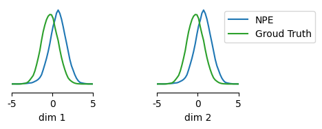
While NPE is not completely off, it does not provide a perfect fit to the posterior. In cases where the likelihood is tractable, we can fix this with importance sampling.

Importance sampling with the SBI toolbox

With the sbi toolbox, importance sampling is a one-liner. sbi supports two methods for importance sampling:

• "importance": returns n_samples weighted samples (as above) corresponding to n_samples * sample_efficiency samples from the posterior. This results in unbiased samples, but the number of effective samples may be small when the sbi estimate is inaccurate.

• "sir" (sampling-importance-resampling): performs rejection sampling on a batched basis with batch size oversampling_factor. This is a guaranteed way to obtain N / oversampling_factor samples, but these may be biased as the weight normalization is not performed across the entire set of samples.

posterior_sir = ImportanceSamplingPosterior(
    potential_fn=log_prob_fn,
    proposal=posterior,
    method="sir",
).set_default_x(observation)

theta_inferred_sir = posterior_sir.sample(
    (1000,),
    oversampling_factor=32,
)

fig, ax = marginal_plot(
    [theta_inferred, theta_inferred_sir, gt_samples],
    limits=[[-5, 5], [-5, 5]],
    figsize=(5, 1.5),
    diag="kde",  # smooth histogram
)
ax[1].legend(["NPE", "NPE-IS", "Groud Truth"], loc="upper right", bbox_to_anchor=[2.0, 1.0, 0.0, 0.0]);

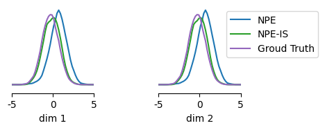
Indeed, the importance-sampled posterior matches the ground truth well, despite significant deviations of the initial NPE estimate.