How to run L-C2ST#
Tests like expected coverage and simulation-based calibration evaluate whether the posterior is on average across many observations well-calibrated. Unlike these tools, L-C2ST allows you to evaluate whether the posterior is correct for a specific observation. While this is powerful, L-C2ST requires to train an additional classifier (which must be trained on sufficiently many new simulations, and its statistical power depends on whether the classifier performs well.
The sbi toolbox implements L-C2ST. Below, we first provide a brief syntax of L-C2ST, followed by a detailed explanation of the mathematical background and a full example.
Main syntax#
from sbi.diagnostics.lc2st import LC2ST

# Simulate calibration data. Should be at least in the thousands.
num_lc2st_samples = 10_000
prior_samples = prior.sample((num_lc2st_samples,))
prior_predictives = simulator(prior_samples)

# Generate one posterior sample for every prior predictive.
post_samples_cal = posterior.sample_batched(
    (1,),
    x=prior_predictives,
    max_sampling_batch_size=10
)[0]

# Train the L-C2ST classifier.
lc2st = LC2ST(
    thetas=prior_samples,
    xs=prior_predictives,
    posterior_samples=post_samples_cal,
    classifier="mlp",
    num_ensemble=1,
)
_ = lc2st.train_under_null_hypothesis()
_ = lc2st.train_on_observed_data()

# Note: x_o must have a batch-dimension. I.e. `x_o.shape == (1, observation_shape)`.
post_samples_star = posterior.sample((10_000,), x=x_o)
probs_data, scores_data = lc2st.get_scores(
    theta_o=post_samples_star,
    x_o=x_o,
    return_probs=True,
    trained_clfs=lc2st.trained_clfs
)
probs_null, scores_null = lc2st.get_statistics_under_null_hypothesis(
    theta_o=post_samples_star,
    x_o=x_o,
    return_probs=True,
)

conf_alpha = 0.05
p_value = lc2st.p_value(post_samples_star, torch.as_tensor(x_o).unsqueeze(0))
reject = lc2st.reject_test(post_samples_star, torch.as_tensor(x_o).unsqueeze(0), alpha=conf_alpha)

fig, ax = plt.subplots(1, 1, figsize=(5, 3))
quantiles = np.quantile(scores_null, [0, 1-conf_alpha])
ax.hist(scores_null, bins=50, density=True, alpha=0.5, label="Null")
ax.axvline(scores_data, color="red", label="Observed")
ax.axvline(quantiles[0], color="black", linestyle="--", label="95% CI")
ax.axvline(quantiles[1], color="black", linestyle="--")
ax.set_xlabel("Test statistic")
ax.set_ylabel("Density")
ax.set_title(f"p-value = {p_value:.3f}, reject = {reject}")
plt.show()
This will return a figure as the following:
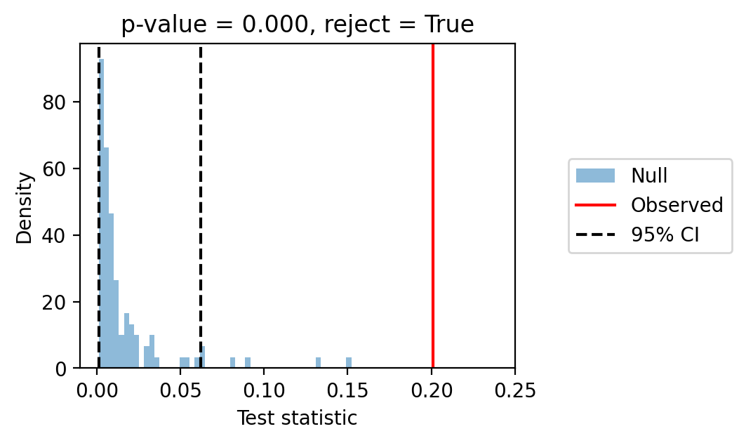
If the red line is outside of the two dotted black lines (as above), then L-C2ST rejects the null-hypothesis that the approximate posterior matches the true posterior (i.e., your posterior is likely wrong).
If the posterior is wrong, then you can get insights into whether the posterior is under- or over-confident as follows:
from sbi.analysis.plot import pp_plot_lc2st

pp_plot_lc2st(
    probs=[probs_data],
    probs_null=probs_null,
    conf_alpha=0.05,
    labels=["Classifier probabilities \n on observed data"],
    colors=["red"],
)
This plots something like the following:
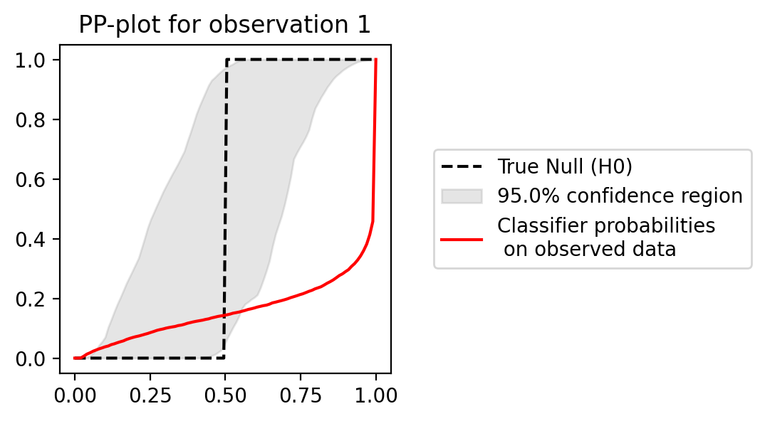
If the red line is below the gray area, then the posterior is over-confident. If the red line is above the gray area, then the posterior is under-confident.
Additional explanation#
For a detailed example and additional explanation, see this tutorial.
Citation#
@article{linhart2023c2st,
  title={L-c2st: Local diagnostics for posterior approximations in simulation-based inference},
  author={Linhart, Julia and Gramfort, Alexandre and Rodrigues, Pedro},
  journal={Advances in Neural Information Processing Systems},
  volume={36},
  pages={56384--56410},
  year={2023}
}