How to detect model misspecification#
“Model misspecification” means that the simulator can, for no parameter set, match the observation. In that case, all methods implemented in sbi will likely perform poorly. As such, it is essential to detect whether the model is misspecified (or, which observations are misspecified, i.e., cannot be captured by the model).
sbi provides two diagnostics for identifying that the model is misspecified. The calc_misspecification_logprob() is useful particularly for low-dimensional simulation outputs. The calc_misspecification_mmd is performed in latent space of the neural network and is most useful for high-dimensional simulation outputs.
Main syntax for calc_misspecification_logprob()#
from sbi.diagnostics.misspecification import calc_misspecification_logprob
from sbi.inference.trainers.marginal import MarginalTrainer

# Generate training data. This can be re-used for NPE or other inference methods.
theta = prior.sample((1000,))
x = simulate(theta)

trainer = MarginalTrainer(density_estimator='NSF')
trainer.append_samples(x)
est = trainer.train()

p_value, reject_H0 = calc_misspecification_logprob(x_train, x_o, est)

plt.figure(figsize=(6, 4), dpi=80)
plt.hist(est.log_prob(x_train).detach().numpy(), bins=50, alpha=0.5, label=r'log p($x_{train}$)')
plt.axvline(est.log_prob(x_o).detach().item(), color="red", label=r'$\log p(x_{o_{mis}})$)')
plt.ylabel('Count')
plt.xlabel(r'$\log p(x)$')
plt.legend()
plt.show()
This will return a plot like the following:
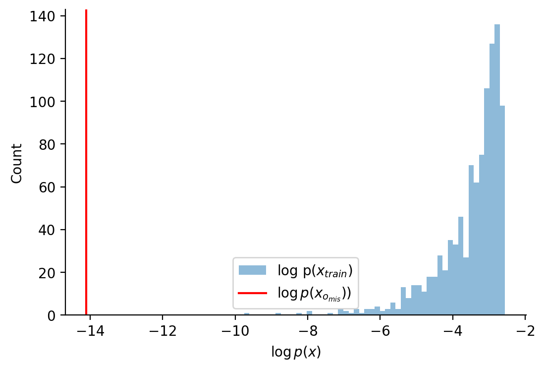
Interpretation: We can clearly see that the log_prob for the misspecified observation x_o_mis is far away from the log_probs of the training data and also that of the well-specified sample x_o. This indicates that the observation is misspecified.
Similarly, p_value is 0.0, which means that we reject the null hypothesis that the observation was generated by the simulator.
Main syntax for calc_misspecification_mmd()#
from sbi.diagnostics.misspecification import calc_misspecification_mmd

# This method needs an embedding network.
density_estimator = posterior_nn("maf", FCEmbedding(20))
inference = NPE(density_estimator=density_estimator)

p_val, (mmds_baseline, mmd) = calc_misspecification_mmd(
    inference=NPE_well_embd, x_obs=x_o_mis, x=x_val_well, mode="embedding"
)

plt.figure(figsize=(6, 4), dpi=80)
plt.hist(mmds_baseline.numpy(), bins=50, alpha=0.5, label="baseline")
plt.axvline(mmd.item(), color="k", label=r"MMD(x, $x_o$)")
plt.ylabel("Count")
plt.xlabel("MMD")
plt.legend()
plt.show()
This will plot:
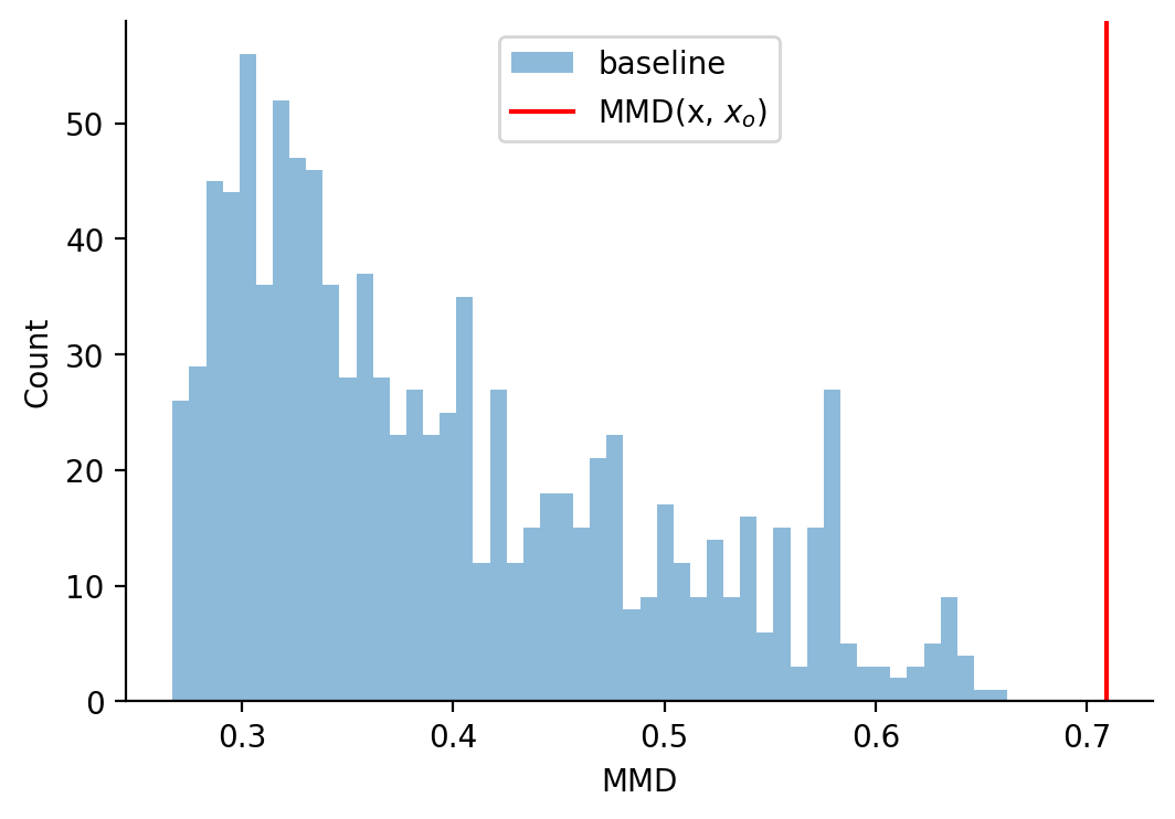
Interpretation: The MMD between x_o and simulated data (black) is outside of the distribution of MMDs between simulated data (blue). This indicates that our simulator is misspecified.
Similarly, the p_val is 0.0 (not shown in the plot), meaning that we reject the null-hypothesis that x_o comes from the distribution defind by the simulator.
Example and more explanation#
If you want to learn more, read the tutorial here.
Citation#
For the MMD-based misspecification metric, please cite:
@inproceedings{schmitt2023detecting,
  title={Detecting model misspecification in amortized Bayesian inference with neural networks},
  author={Schmitt, Marvin and B{\"u}rkner, Paul-Christian and K{\"o}the, Ullrich and Radev, Stefan T},
  booktitle={DAGM German Conference on Pattern Recognition},
  pages={541--557},
  year={2023},
  organization={Springer}
}
The method based on training an unconditional density estimator is unpublished, please just cite the sbi toolbox for it.