How to run TARP#
TARP is an alternative calibration check proposed recently in https://arxiv.org/abs/2302.03026.
In contrast to SBC (Talts et al.) and expected coverage based highest posterior density regions (Deistler et al.,), TARP provides a necessary and sufficient condition for posterior accuracy, i.e., it can also detect inaccurate posterior estimators.
Note, however, that this property depends on the choice of reference point distribution: to obtain the full diagnostic power of TARP, one would need to sample reference points from a distribution that depends on \(x\). Thus, in general, we recommend using and interpreting TARP like SBC and complementing coverage checks with posterior predictive checks.
You can run TARP in the sbi toolbox as follows:
from sbi.diagnostics import run_tarp, check_tarp
from sbi.analysis.plot import plot_tarp

posterior = inference.build_posterior()

num_tarp_samples = 200  # choose a number of sbc runs, should be ~100s
# generate ground truth parameters and corresponding simulated observations for SBC.
prior_samples = prior.sample((num_tarp_samples,))
prior_predictives = simulator(thetas)

# the tarp method returns the ECP values for a given set of alpha coverage levels.
ecp, alpha = run_tarp(
    prior_samples,
    prior_predictives,
    posterior,
    references=None,  # will be calculated automatically.
    num_posterior_samples=1000,
    use_batched_sampling=False,  # `True` can give speed-ups, but can cause memory issues.
)
# Similar to SBC, we can check then check whether the distribution of ecp is close to
# that of alpha.
atc, ks_pval = check_tarp(ecp, alpha)
print(atc, "Should be close to 0")
print(ks_pval, "Should be larger than 0.05")

plot_tarp(ecp, alpha)
This generates a plot like the following:
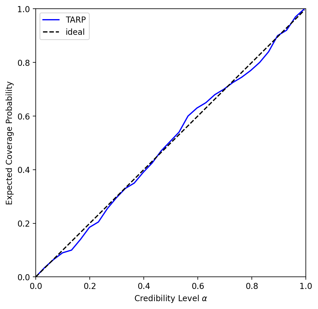
If the blue curve is above the diagonal, then the posterior estimate is under-confident. If it is under the diagonal, then the posterior estimate is over confident.
Explanation#
Given a test set \((\theta^*, x^*)\) and a set of reference points \(\theta_r\), TARP calculates statistics for posterior calibration by
drawing posterior samples \(\theta\) given each \(x_*\)
calculating the distance \(r\) between \(\theta_*\) and \(\theta_r\)
counting for how many of the posterior samples their distance to \(\theta_r\) is smaller than \(r\)
See https://arxiv.org/abs/2302.03026, Figure 2, for an illustration.
For each given coverage level \(\alpha\), one can then calculate the corresponding average counts and check, whether they correspond to the given \(\alpha\).
Citation#
@inproceedings{lemos2023sampling,
  title={Sampling-based accuracy testing of posterior estimators for general inference},
  author={Lemos, Pablo and Coogan, Adam and Hezaveh, Yashar and Perreault-Levasseur, Laurence},
  booktitle={International Conference on Machine Learning},
  pages={19256--19273},
  year={2023},
  organization={PMLR}
}