Vector Field Methods: FMPE and NPSE

sbi incorporates recent algorithms based on Flow Matching and Score Matching generative models, which are also referred to as Continuous Normalizing Flows (CNF) and Denoising Diffusion Probabilistic Models (DDPM), respectively.

At the highest level, you can think of FMPE and NPSE as solving the same problem as NPE, i.e., estimating the posterior from simulations, but replacing Normalizing Flows with different conditional density estimators.

Flow Matching and Score Matching, as generative models, are also quite similar to Normalizing Flows, where a deep neural network parameterizes the transformation from a base distribution (e.g., Gaussian) to a more complex one that approximates the target density. In essence, they differ in how they model this transformation, namely by modeling the vector field of the transformation.

Additionally, Flow Matching and Score Matching offer different benefits and drawbacks compared to Normalizing Flows, which make them better (or worse) choices for some problems. For example, Score Matching (Diffusion Models) are known to be very flexible and can model high-dimensional distributions, but are comparatively slow during sampling.

When to use vector field methods over NPE

	NPE (normalizing flows)	FMPE / NPSE
Architecture	Restricted to invertible transforms	Any neural network
Sampling speed	Fast (single forward pass)	Slower (ODE/SDE integration)
Scalability	Limited in very high dims	Better scaling to high dims
Multi-round	Fully supported	Single-round only
Log-prob	Exact, fast	Via ODE or SDE (slower)

References

Score Matching:

• Hyvärinen, A. “Estimation of Non-Normalized Statistical Models by Score Matching.” JMLR 2005.

• Song, Y., et al. “Score-Based Generative Modeling through Stochastic Differential Equations.” ICLR 2021.

• Geffner, T., et al. “Score modeling for simulation-based inference.” ICML 2023.

• Sharrock, L., et al. “Sequential neural score estimation.” ICML 2024.

• Karras, T., et al. “Elucidating the Design Space of Diffusion-Based Generative Models.” NeurIPS 2022.

• Linhart, J., et al. “Diffusion posterior sampling for simulation-based inference in tall data settings.” 2024.

Flow Matching:

• Lipman, Y., et al. “Flow Matching for Generative Modeling.” ICLR 2023.

• Wildberger, J.B., et al. “Flow Matching for Scalable Simulation-Based Inference.” NeurIPS 2023.

1. Setup

We use a simple 3D linear Gaussian simulator throughout this tutorial.

import torch

from sbi.analysis import pairplot
from sbi.inference import FMPE, NPSE
from sbi.neural_nets import posterior_flow_nn, posterior_score_nn
from sbi.utils import BoxUniform

# Define prior and simulator
num_dims = 3
num_sims = 10000
num_posterior_samples = 1000
prior = BoxUniform(low=-torch.ones(num_dims), high=torch.ones(num_dims))
labels = [r"$\theta_1$", r"$\theta_2$", r"$\theta_3$"]

def simulator(theta):
    """Linear Gaussian simulator."""
    return theta + 1.0 + torch.randn_like(theta) * 0.1

# Generate training data
theta = prior.sample((num_sims,))
x = simulator(theta)

# Ground truth observation
theta_o = torch.zeros(num_dims)
x_o = simulator(theta_o)

2. FMPE — Flow Matching Posterior Estimation

Flow-Matching Posterior Estimation (FMPE) is an approach to SBI that leverages Flow Matching, a generative modeling technique where the transformation from a simple base distribution (like a Gaussian) to the target distribution is learned through matching the flow of probability densities.

The core idea is to model the probability flow between the base distribution and the target distribution by training a neural network to parameterize a velocity field that defines how samples should be moved or transformed. As such, they learn a continuous time flow between the source and target distribution and are also referred to as continuous-time normalizing flows. The velocity field can be represented by an ODE and sampling from and evaluation the target distribution then amounts to solving the ODE forward or backward in time.

Step-by-Step Process

1. Base Distribution: Start with a simple base distribution (e.g., Gaussian).

2. Neural Network Parameterization: Use a neural network to learn a vector field that describes the flow from the base distribution to the target distribution.

3. Flow Matching Objective: Optimize the neural network to minimize a loss function that captures the difference between the learned and target vector fields.

4. Sampling: Once trained, draw samples from the base distribution and apply the learned flow transformation by solving an ODE to obtain samples from the approximate posterior.

FMPE can be more efficient than traditional normalizing flows in some settings, especially when the target distribution has complex structures or when high-dimensional data is involved (see Dax et al., 2023 for an example). However, compared to discrete-time normalizing flows, flow matching is usually slower at inference time because sampling requires solving the underlying ODE (compared to just doing a NN forward pass for normalizing flows).

Key properties:

• Default sampling: sample_with="ode" (fast, deterministic)

• Through the conceptual and mathematical connection to score matching (see below), it also supports sampling via an SDE.

# Minimal FMPE example
fmpe_trainer = FMPE(prior)
fmpe_trainer.append_simulations(theta, x).train()
fmpe_posterior = fmpe_trainer.build_posterior()
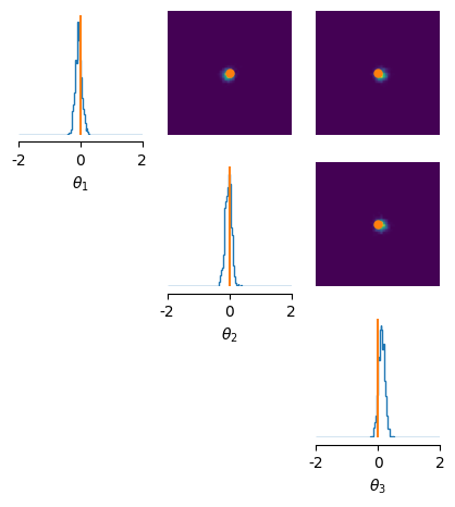
samples_fmpe = fmpe_posterior.sample((num_posterior_samples,), x=x_o)

fig, ax = pairplot(
    samples_fmpe, limits=[[-2, 2]] * 3, figsize=(5, 5),
    labels=labels,
    points=theta_o,
)

 Neural network successfully converged after 114 epochs.

3. NPSE — Neural Posterior Score Estimation

NPSE approximates a target posterior distribution \(p_0(\theta|x_0)\) by learning its score function, i.e., the gradient of the log-density of the (diffused) posterior \(\nabla_{\theta}\log p_t(\theta|x)\), for all times \(t\) and all conditional observations \(x\), using the denoising score matching loss. Score-based generative models are closely linked to diffusion models, especially during the sampling phase.

The core idea of diffusion models is that one can learn complex distributions from data by gradually adding noise to the data until it is pure noise (e.g., a Gaussian), while learning the mathematical representation of these noise additions (the score function) along the way. Crucially, there is a mathematical way to also represent the reverse direction, i.e., the denoising steps. Therefore, after training, one can also start with as simple noise distribution and obtain samples from the target distribution by gradually applying the learnt denoising steps.

Sampling from the target posterior \(p_0(\theta|x_0)\) can be split into two steps: - Forward step: Diffuse samples from \(p_0(\theta|x_0)\) over time and learn the diffused scores \(\nabla_{\theta}\log p_t(\theta|x)\) for all \(t \in [0, t_{\max}]\). At the end (\(t=t_{\max}\)), the diffused posterior is close to a standard Gaussian. - Reverse step: Reverse the diffusion process, starting from a standard Gaussian, using the learned scores to generate new samples from \(p_0(\theta|x_0)\).

Score-based generative models have been shown to scale well to very high dimensions (e.g., high-resolution images), which is particularly useful when the parameter space is high-dimensional. On the other hand, sampling can be slower as it involves solving many steps of the stochastic differential equation for reversing the diffusion process.

For more details on score-based generative models, see Song et al., 2020 (in particular, Figures 1 and 2).

Note that only the single-round version of NPSE is implemented currently.

In sbi, the sde_type parameter defines whether the forward diffusion process has a noising schedule that is Variance Exploding ("ve", i.e., SMLD), Variance Preserving ("vp", i.e., DDPM), or sub-Variance Preserving ("subvp").

# Minimal NPSE example
npse_trainer = NPSE(prior, sde_type="ve")
npse_trainer.append_simulations(theta, x).train()
npse_posterior = npse_trainer.build_posterior()
samples_npse = npse_posterior.sample((num_posterior_samples,), x=x_o)

fig, ax = pairplot(
    samples_npse, limits=[[-2, 2]] * 3, figsize=(5, 5),
    labels=labels,
    points=theta_o,
)

 Neural network successfully converged after 170 epochs.

4. Network Architectures

While NPE is architecturally limited to conditional density networks (normalizing flows), both FMPE and NPSE solve a regression problem targeting a specific vector field (e.g., marginal scores or transport velocities). This is advantageous because it allows us to use any “off-the-shelf” neural network, in contrast to NPE, which is typically restricted to normalizing flows.

However, performance can be highly dependent on the suitability of the chosen neural network for the task at hand. For instance, diffusion models achieve state-of-the-art generative performance on images only when paired with a carefully designed U-Net-like architecture.

For both FMPE and NPSE, we provide a selection of neural networks tailored to the task:

• "mlp" and "ada_mlp" (MLP with adaptive layer norm for conditioning) — MLP variants that inject time information at each layer, as is common in diffusion architectures.

• "transformer" and "transformer_cross_attn" — scalable diffusion transformers (e.g., as in Peebles & Xie, 2023). The cross-attention variant supports arbitrary sequence lengths for conditioning.

For certain data types, such as image-like inputs, it may still be beneficial to use a more specialized architecture.

Use posterior_flow_nn() for FMPE and posterior_score_nn() for NPSE to configure the network.

# FMPE with a transformer architecture
net_builder = posterior_flow_nn(
    model="transformer",
    num_layers=2,
    num_heads=2,
    hidden_features=64,
)
trainer = FMPE(prior, vf_estimator=net_builder)
estimator = trainer.append_simulations(theta, x).train(
    training_batch_size=200, learning_rate=5e-4
)

 Neural network successfully converged after 123 epochs.

# NPSE with custom network configuration via posterior_score_nn
net_builder = posterior_score_nn(
    model="mlp",
    sde_type="ve",
    hidden_features=128,
    num_layers=6,
)
trainer = NPSE(prior, vf_estimator=net_builder)
estimator = trainer.append_simulations(theta, x).train()

 Neural network successfully converged after 87 epochs.

Custom networks via the VectorFieldNet protocol

You can use your custom network for estimating the vector field, essentially any torch.nn.Module that follows the VectorFieldNet protocol: it must accept (theta, x, t) and return a tensor with the same shape as theta.

from sbi.utils.vector_field_utils import VectorFieldNet


class CustomNet(VectorFieldNet):
    def __init__(self):
        super().__init__()
        self.layers = torch.nn.Sequential(
            torch.nn.Linear(3 + 3 + 1, 128),  # theta_dim + x_dim + 1; adapt these to your problem
            torch.nn.GELU(),
            torch.nn.Linear(128, 128),
            torch.nn.GELU(),
            torch.nn.Linear(128, 3),  # must match theta_dim
        )

    def forward(self, theta, x, t):
        h = torch.cat([theta, x, t[..., None]], dim=-1)
        return self.layers(h)

# Wrap in the factory function (adds z-scoring).
net_builder = posterior_flow_nn(model=CustomNet())
trainer = FMPE(prior, vf_estimator=net_builder)
estimator = trainer.append_simulations(theta, x).train()

 Neural network successfully converged after 160 epochs.

5. Noise Schedules and Training Options

In score matching, the noise schedule defines the way we add noise to the target data across time. Per default, this noise is added uniformly across time. However, it has been shown that for some problems performance can be improved by having a dedicated noise schedule that is not uniform across time Karras et al. 2022. In sbi we therefore implemented an option to pass different noise schedules for the NPSE training phase and the sampling phase.

All SDE types have tunable noise range parameters:

• VE: sigma_min / sigma_max (default: 1e-4, 10.0) — controls the range of noise added during diffusion.

• VP / SubVP: beta_min / beta_max (default: 0.01, 10.0) — controls the linear noise schedule.

These can be passed as **kwargs to posterior_score_nn() and are validated by ScoreEstimatorConfig.

EDM-style time sampling schedules (VE only)

For NPSE with sde_type="ve", you can use EDM-style schedules from Karras et al. 2022:

• train_schedule="lognormal": Concentrates training on intermediate noise levels where the score is most informative.

• solve_schedule="power_law": Concentrates sampling steps near low noise levels for sharper samples.

# NPSE with EDM-style noise schedules
net_builder = posterior_score_nn(
    model="mlp",
    sde_type="ve",
    # EDM-style training schedule
    train_schedule="lognormal",
    lognormal_mean=-1.2,
    lognormal_std=1.2,
    # EDM-style solving schedule
    solve_schedule="power_law",
    power_law_exponent=7.0,
    # Noise range
    sigma_min=1e-3,  # default: 1e-4
    sigma_max=15.0,  # default: 10.0; increased for broader prior
)
trainer = NPSE(prior, vf_estimator=net_builder)
trainer.append_simulations(theta, x).train()
posterior = trainer.build_posterior()

 Neural network successfully converged after 196 epochs.

6. A bridge between FMPE and NPSE. Sampling with SDE vs ODE

It has been shown that a under trained flow matching model (FMPE) implicitly defines a score function, and therefore also an SDE that can be used for stochastic sampling, exactly like NPSE Singh et al., 2024. This can be useful for SBI because SDE-based score methods have some additional benefits over FMPE, e.g., sampling complex posterior shapes, posterior sampling given i.i.d. data, or guidance (see below).

Practially in sbi this implies that both FMPE and NPSE support both SDE and ODE sampling. Per default FMPE uses sample_with="ode" (deterministic, fast) and NPSE uses sample_with="sde" (stochastic, more robust). However, The sample_with argument allows you to choose which kind of solver to use to reverse the diffusion equation:

• "ode": Builds the probability flow ODE using the zuko library. Sampling is deterministic and typically faster.

• "sde": Solves the reverse SDE by alternating prediction and correction steps. The only available predictor is "euler_maruyama" and the available correctors are "langevin" (for Unadjusted Langevin Dynamics) and "gibbs" (for Gibbs sampling).

Both options include rejection sampling steps to ensure samples remain within the prior support.

For SDE sampling, you can configure:

• predictor: Integration scheme (default: "euler_maruyama")

• corrector: Optional correction step (None, "langevin", "gibbs")

• steps: Number of integration steps (default: 500)

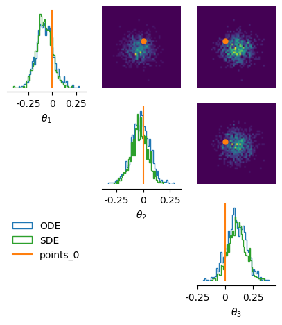
# We can sample from a FMPE posterior using ODE or SDE sampling.
# ODE sampling (faster, deterministic)
posterior_ode = fmpe_trainer.build_posterior(estimator, sample_with="ode")
samples_ode = posterior_ode.sample((num_posterior_samples,), x=x_o)

# SDE sampling (stochastic, can be more robust)
posterior_sde = fmpe_trainer.build_posterior(estimator, sample_with="sde")
samples_sde = posterior_sde.sample((num_posterior_samples,), x=x_o)

fig, axes = pairplot(
    [samples_ode, samples_sde],
    figsize=(5, 5),
    labels=labels,
    points=theta_o,
    legend=True,
    samples_labels=["ODE", "SDE"],
)

7. MAP Estimation

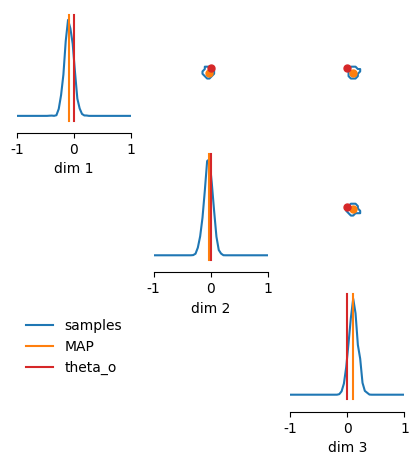
It is possible to get a Maximum A Posteriori (MAP) estimate with both FMPE and NPSE. The optimization procedure (gradient ascent) finds a maximizer \(\theta_{\max}\) of the posterior log-probability \(\log p(\theta|x_0)\).

The default values (number of optimization steps, starting positions, learning rate) might require hand-tuning for your problem.

Note that MAP does not differentiate through the full log-prob ODE (which would be very expensive). Instead, it uses the network’s score estimate at \(t_{\min}\) directly for gradient ascent (the network has already learned this gradient during training).

# MAP estimation (works for both FMPE and NPSE)
fmpe_posterior = fmpe_posterior.set_default_x(x_o)

map_estimate = fmpe_posterior.map(num_iter=50, learning_rate=0.01, show_progress_bars=True)

 Optimizing MAP estimate. Iterations: 95 / 100. Performance in iteration 0: 4.02 (= unnormalized log-prob). Press Ctrl-C to interrupt.Optimization was interrupted after 95 iterations. 

# Plot posterior samples and MAP
fig, ax = pairplot(
    samples_sde,
    figsize=(5, 5),
    limits=[[-1, 1]] * 3,
    diag = "kde",
    upper="contour",
    diag_kwargs=dict(bins=100),
    upper_kwargs=dict(levels=[0.95]),
    points=[map_estimate, theta_o.unsqueeze(0)], # add ground truth thetas and MAP
    points_labels=["MAP", "theta_o"],
    samples_labels=["samples"],
    legend=True,
)

8. Batched Sampling

Given a batch of observations \([x_1, \ldots, x_B]\) (not i.i.d.), it is possible to get samples from posteriors \(p(\theta|x_1)\), …, \(p(\theta|x_B)\) in a vectorized manner without retraining! This is implemented in the sample_batched() method. The argument sample_shape specifies the desired number of samples for each posterior.

# Generate a batch of observations
x_batch = simulator(prior.sample((5,)))  # 5 different observations

# Batched sampling: returns shape (num_samples, num_observations, num_dims)
samples_batch = fmpe_posterior.sample_batched(
    sample_shape=(1_000,),
    x=x_batch,
)
print(f"Batched samples shape: {samples_batch.shape}")

Batched samples shape: torch.Size([1000, 5, 3])

9. IID / Tall Posteriors

When \(x_0\) is a batch of i.i.d. observations \(x_0 = [x_0^0, \ldots, x_0^N]\), it is possible to sample from the tall posterior distribution \(p(\theta|x_0^0, \ldots, x_0^N)\) by aggregating the i.i.d. observations on the score-level (Geffner et al., 2023). Thanks to the FMPE-NPSE bridge, this also works for FMPE by switching the SDE at inference / sampling time.

Once the score/velocity estimate is trained, sampling from \(p(\theta|x_0^0, \ldots, x_0^N)\) is split into two steps:

1. Estimate the scores of the tall posterior for all times \(t\), based on the learned scores of individual posteriors \(p(\theta|x_0^i)\).

2. Reverse the diffusion process or solve the SDE using the estimated scores.

To sample, call .sample() as before but pass a batch of observations to x — the algorithm will assume those to be i.i.d. and automatically switch to the tall posterior setting.

The iid_method argument specifies the method used to estimate the scores of the tall posterior using the individual posterior scores:

• "auto_gauss" (recommended): Auto-calibrates Gaussian approximation of the marginal score. Has initial overhead but is accurate and robust. See Linhart et al., 2024.

• "gauss": Faster Gaussian approximation, good for simple problems. See Linhart et al., 2024.

• "jac_gauss": Most accurate, uses iterative Jacobian computations (expensive). See Linhart et al., 2024.

• "fnpe": Factorized Neural Posterior Estimation — simple and fast, but can become inaccurate for many observations due to heuristic approximations. See Geffner et al., 2023.

# Re-use the NPSE posterior trained on single observations from above.
posterior = npse_trainer.build_posterior(sample_with="sde")

# Generate i.i.d. observations from the same ground truth
num_iid_samples = 10
x_iid = torch.stack([simulator(theta_o) for _ in range(num_iid_samples)])

# Sample from the tall posterior
samples_iid = posterior.sample(
    (num_posterior_samples,), x=x_iid,
    iid_method="auto_gauss",
)

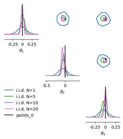
Progressive sharpening with more observations

The posterior concentrates around the true parameter as the number of i.i.d. observations increases.

# Compare posteriors with different numbers of i.i.d. observations
x_iid_20 = torch.stack([simulator(theta_o) for _ in range(20)])
all_samples = []
labels = []
for n_obs in [1, 5, 10, 20]:
    x_subset = x_iid_20[:n_obs]
    samples = posterior.sample((1_000,), x=x_subset)
    all_samples.append(samples)
    labels.append(f"N={n_obs}")

fig, axes = pairplot(
    all_samples,
    figsize=(5, 5),
    points=theta_o.unsqueeze(0),  # add batch dimension for plotting
    points_colors=["k"],
    labels=[r"$\theta_1$", r"$\theta_2$", r"$\theta_3$"],
    diag="kde",
    upper="contour",
    upper_kwargs=dict(levels=[0.99]),
    points_offdiag=dict(markersize=5),
    legend=True,
    samples_labels=[f"i.i.d. N={n}" for n in [1, 5, 10, 20]],
);

10. Guidance Methods

Guidance methods allow post-hoc modifications to the posterior without retraining. The core idea is that the learned posterior score can be decomposed into a prior score and a likelihood score. Since we know the prior analytically, we can compute the prior score at any diffusion time in closed form, and then obtain the likelihood score as the difference between the learned posterior score and the prior score. Once decomposed, we can independently modify each component — for example, scaling up the likelihood score to sharpen the posterior, or swapping the prior score for a different prior — and then recombine them for sampling. This is powerful for SBI because it means you train once and can then adjust the posterior at inference time for different priors, sharper or flatter posteriors, or addi

Thus, if we want to do certain modifications to our model after training, e.g.:

• Shifting prior/likelihood location/scale.

• Truncating the prior.

• Changing the prior to a different distribution,

then diffusion-based guidance is a way to do so. In sbi, we implemented several guidance methods to perform such operations. Note that guidance affects .sample() only, .log_prob() and .map() are not supported with active guidance.

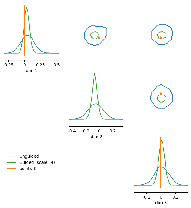
Affine Classifier-Free Guidance

The following classifier-free guidance method allows you to scale and shift the prior and likelihood score contributions. This can be used to perform “super” conditioning, i.e., shrink the variance of the likelihood:

# Affine classifier-free guidance: sharpen the posterior
from torch.distributions import MultivariateNormal

# Train with Gaussian prior.
prior = MultivariateNormal(loc=torch.zeros(num_dims), covariance_matrix=torch.eye(num_dims))
theta = prior.sample((num_sims,))
x = simulator(theta)
trainer = NPSE(prior)
trainer.append_simulations(theta, x).train()
posterior = trainer.build_posterior(sample_with="sde")
theta_o = torch.zeros(num_dims)
x_o = simulator(theta_o)

# Guidance parameters: increase likelihood scale to sharpen the posterior
guidance_params = {
    "likelihood_scale": 4.0,  # increase the likelihood precision (-> narrower posterior)
    "prior_scale": 1.,  # same prior precision
    "prior_shift": 0.,  # same prior mean
    "likelihood_shift": 0.,  # same likelihood mean
}

# Unguided
samples_unguided = posterior.sample((1_000,), x=x_o)

# Guided: increase likelihood scale to sharpen, no re-training.
samples_guided = posterior.sample(
    (1_000,), x=x_o,
    guidance_method="affine_classifier_free",
    guidance_params=guidance_params,
)

fig, axes = pairplot(
    [samples_unguided, samples_guided],
    figsize=(8, 8),
    diag="kde",
    upper="contour",
    upper_kwargs=dict(levels=[0.99]),
    points=theta_o.unsqueeze(0),
    legend=True,
    samples_labels=["Unguided", "Guided (scale=4)"],
)

 Neural network successfully converged after 91 epochs.

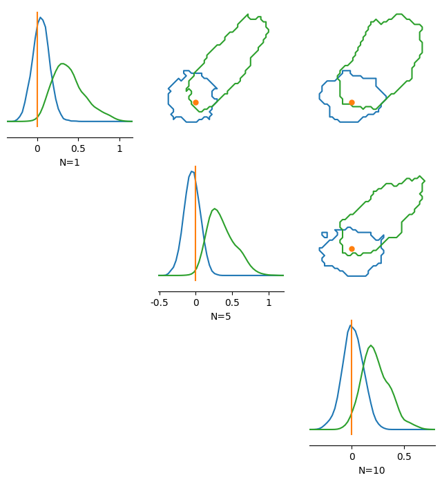
Prior Guidance

A more general method is prior guidance, which allows you to specify arbitrary training and test priors (see Yang et al., 2025). The only requirement is that the test prior should be covered by the training prior — otherwise the guidance will push samples outside the training distribution where the score estimates will be poor.

Note that when using a shifted or correlated test prior, the original ground truth \(\theta_o\) may lie outside the guided posterior’s mass. This is expected, as \(\theta_o\) was generated under the training prior.

Below we exchange the training prior (standard normal) for a shifted multivariate normal prior with correlations:

from torch.distributions import MultivariateNormal

# Broad prior from above.
train_prior = prior

# Test with a shifted, correlated prior
test_prior = MultivariateNormal(
    loc=torch.zeros(num_dims) + 0.1,
    covariance_matrix=torch.tensor([[0.5, 0.3, 0.1],
                      [0.3, 0.4, 0.2],
                      [0.1, 0.2, 0.3]])
)

# For more complicated adjustments we need a larger K (number of mixture components for
# approximating the prior).
guidance_params = {
    "test_prior": test_prior,
    "train_prior": train_prior,
    "K": 8,
    "covariance_type": "full"  # Required for adding new correlations!
}

# No need to train again, just plug in the new guidance parameters when sampling.
samples_prior_guided = posterior.sample(
    (1_000,),
    x=x_o,
    guidance_method="prior_guide",
    guidance_params=guidance_params,
)

pairplot(
    [samples_unguided, samples_prior_guided],
    points=theta_o.unsqueeze(0),
    figsize=(8, 8),
    diag="kde",
    upper="contour",
    upper_kwargs=dict(levels=[0.99]),
    labels=labels,
);

Summary

Feature	FMPE	NPSE
What it learns	Velocity field	Score function
Default sampling	ODE	SDE
SDE types	N/A	"ve", "vp", "subvp"
Noise range params	N/A	sigma_min/max (VE), beta_min/max (VP)
EDM schedules	N/A	train_schedule, solve_schedule
MAP estimation	Yes	Yes
Batched sampling	Yes	Yes
IID posteriors	Yes	Yes
Guidance	Yes	Yes
Multi-round	Not supported	Not supported

For practical guidance on choosing between options, see the how-to guide: How to Choose Vector Field Options.